Decoding the holograph of functional cell-cell communication events

Following the first tutorial, in this tutorial, we demonstrate how HoloNet can be used to decode the holograph of functional cell-cell communication events (FCEs) in spatial transcriptomics data.

For each downstream target gene, HoloNet:

• Identifies cell types serving as major senders

• Identifies ligand–receptor pairs serving as core mediators

in FCEs for specific downstream genes.

Note

The tutorial mainly follows these steps:

1. Load data and construct multi-view communication event (CE) network

2. Predict specific target gene expression.

3. Decode the FCEs for the gene by interpreting the trained model.

4. Identify genes more affected by cell–cell communication.

import HoloNet as hn

import os
import pandas as pd
import numpy as np
import scanpy as sc
import matplotlib.pyplot as plt
import torch

import warnings
warnings.filterwarnings('ignore')
hn.set_figure_params(tex_fonts=False)
sc.settings.figdir = './figures/'

Data loading and constructing multi-view CE network

Just like the first tutorial, load the example breast cancer dataset:

adata = hn.pp.load_brca_visium_10x()

Load the ligand-receptor (LR) pair database and filter the LR pair:

interaction_db, cofactor_db, complex_db = hn.pp.load_lr_df(human_or_mouse='human')
expressed_lr_df = hn.pp.get_expressed_lr_df(interaction_db, complex_db, adata)
expressed_lr_df.shape

(325, 12)

Just like the first tutorial, we use HoloNet.tools.default_w_visium() getting a default w_best value.

Then build multi-view CE network using HoloNet.tools.compute_ce_tensor() and HoloNet.tools.filter_ce_tensor().

w_best = hn.tl.default_w_visium(adata)
elements_expr_df_dict = hn.tl.elements_expr_df_calculate(expressed_lr_df, complex_db, cofactor_db, adata)
ce_tensor = hn.tl.compute_ce_tensor(expressed_lr_df, w_best, elements_expr_df_dict, adata)
filtered_ce_tensor = hn.tl.filter_ce_tensor(ce_tensor, adata, expressed_lr_df, elements_expr_df_dict, w_best)

100%|██████████| 325/325 [00:30<00:00, 10.74it/s]
100%|██████████| 325/325 [2:16:41<00:00, 25.24s/it]

Predicting the target gene expression using a graph model

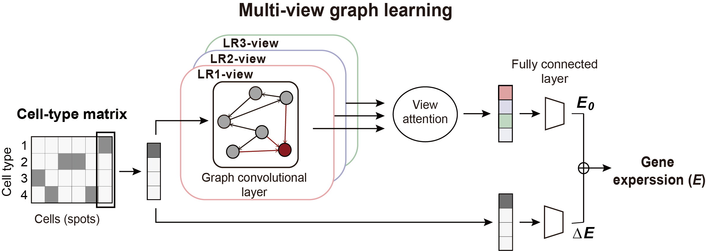
We construct a multi-view graph learning model to predict the expression of gene on interest.

Selecting the target gene to be predicted

Firstly, we select the target genes to be predicted.

The genes with too low, too sparse or too average expression are filtered out. The filtering parameters can be changed in HoloNet.predicting.get_gene_expr().

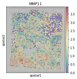
Then we select MMP11, a gene related to tumor invasion as an example target gene.

target_all_gene_expr, used_gene_list = hn.pr.get_gene_expr(adata, expressed_lr_df, complex_db)

target = hn.pr.get_one_case_expr(target_all_gene_expr, cases_list=used_gene_list,
                                 used_case_name='MMP11')
sc.pl.spatial(adata, color=['MMP11'], cmap='Spectral_r', size=1.4, alpha=0.7)

Getting inputs of the graph model

In the multi-view graph learning model, we:

• Use the cell-type matrix as the feature matrix.

• Use normalized multi-view CE network as the adjacency matrix.

Get the feature matrix and adjacency matrix:

X, cell_type_names = hn.pr.get_continuous_cell_type_tensor(adata, continuous_cell_type_slot = 'predicted_cell_type',)
adj = hn.pr.adj_normalize(adj=filtered_ce_tensor, cell_type_tensor=X, only_between_cell_type=True)

If selecting to use categorical cell-type labels, the feature matrix can be derived from HoloNet.predicting.get_one_hot_cell_type_tensor().

Training the graph model

The we train the graph model to predict MMP11 expression. If GPU is avaiable, you can set the device parameter as ‘gpu’. Otherwise, we use CPU by default. The predicted MMP11 expression pattern are similar to the true pattern.

trained_MGC_model_MMP11_list = hn.pr.mgc_repeat_training(X, adj, target, device='gpu')
predict_result_MMP11 = hn.pl.plot_mgc_result(trained_MGC_model_MMP11_list, adata, X, adj)
np.corrcoef(predict_result_MMP11.T, target.T)[0,1]

100%|██████████| 50/50 [01:51<00:00,  2.23s/it]
100%|██████████| 50/50 [00:00<00:00, 85.33it/s]

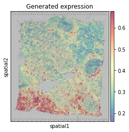
0.5677412923581358

If GPU is not available, you can set repeat_num as a lower number to make the training faster.

Note

The parameters of plotting functions in this tutorials are mainly inherited from two base plotting functions:

• HoloNet.plotting.feature_plot()

• HoloNet.plotting.cell_type_level_network()

Decode the FCEs for the gene by interpreting the trained model

After training the graph model and find the predicted expression profile similar to the true one, we can interprete the trained model to reveal the holography of FCEs.

For each target gene, there are three main output figure:

• LR rank

  • Identify ligand–receptor (LR) pairs serving as core mediators in FCEs for the target gene.

• Cell-type-level FCE network

  • Identifies cell types serving as major senders

  • The cell-type-level FCE network can be LR-pair-specific or general.

• Delta E proportion in each cell-type

  • Identify target gene expression in which cell-types are more dominated by FCEs.

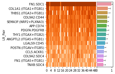
LR rank

Plot the top 15 LR pairs (15 can be changed using plot_lr_num parameter) with the highest view attention weights The heatmap displays the attention weights of each view obtained from repeated training for 50 times. The bar plot represents the mean values of the attention weights of each view.

ranked_LR_df_for_MMP11 = hn.pl.lr_rank_in_mgc(trained_MGC_model_MMP11_list, expressed_lr_df,
                                              plot_cluster=False, repeat_attention_scale=True)

If you want plot the LR-pair clustering results in the LR rank plot, you can set cluster_col=True and provide clustering results in expressed_LR_df.

LR pair clustering can see the first tutorial and HoloNet.tools.cluster_lr_based_on_ce().

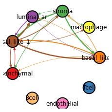
Cell-type-level FCE network

Cell-type-level POSTN:PTK7 FCE network for MMP11. The thickness of the edge represents the strength of POSTN:PTK7 FCEs between the two cell types. The network are derived from interpreting the graph convolutional layer.

In the plot, you can focus on one cell-type and look the edges targeted on it, in order to identify which cell-types are the major sender for it.

_ = hn.pl.fce_cell_type_network_plot(trained_MGC_model_MMP11_list, expressed_lr_df, X, adj,
                                     cell_type_names, plot_lr='FN1:SDC1', edge_thres=0.2,
                                     palette=hn.brca_default_color_celltype,)

100%|██████████| 50/50 [00:00<00:00, 732.48it/s]

If plot_lr is one of the LR pair in the expressed_LR_df, HoloNet.plotting.fce_cell_type_network_plot() will plot the cell-type-level FCE network for a specific LR pair. If plot_lr='all', it will plot the general cell-type-level FCE network for all LR pairs.

Delta E proportion in each cell-type

Identify target gene expression in which cell-types are more dominated by FCEs.

The ratio of the expression change caused by CEs (ΔE) to the sum of ΔE and the baseline MMP11 expression (E0) in each cell type.

delta_e = hn.pl.delta_e_proportion(trained_MGC_model_MMP11_list, X, adj,
                                    cell_type_names,
                                    palette = hn.brca_default_color_celltype)

100%|██████████| 50/50 [00:16<00:00,  3.12it/s]

Identify genes more affected by cell–cell communication

We train the graph model for all selected target genes. (HoloNet.predicting.get_gene_expr() select target gene to be predicted)

Comparing with prediction only using cell-type information, the target with higher performance improvement after considering CEs can be regarded as the genes more affected by cell–cell communication.

trained_MGC_model_only_type_list, \
trained_MGC_model_type_GCN_list = hn.pr.mgc_training_for_multiple_targets(X, adj, target_all_gene_expr, device='gpu')

100%|██████████| 586/586 [2:26:12<00:00, 14.97s/it]

Note

The training process will take a lot of time, you can select to:

• Change the parameters in HoloNet.predicting.get_gene_expr() to obtain less target genes to be predicted.

• Use HoloNet.predicting.save_model_list() in the next section to save the trained model.

Get the predicting results of all target genes:

predicted_expr_type_GCN_df = hn.pr.get_mgc_result_for_multiple_targets(trained_MGC_model_type_GCN_list,
                                                                        X, adj,
                                                                        used_gene_list, adata)
predicted_expr_only_type_df = hn.pr.get_mgc_result_for_multiple_targets(trained_MGC_model_only_type_list,
                                                                        X, adj,
                                                                        used_gene_list, adata)

100%|██████████| 586/586 [03:56<00:00,  2.47it/s]
100%|██████████| 586/586 [03:10<00:00,  3.07it/s]

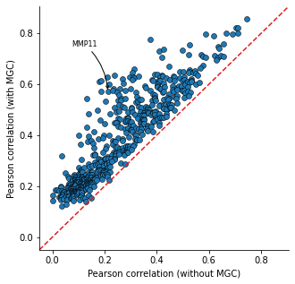
Calculate the Pearson correlation between the predicted expression and the true expression. Compare the correlation from model only using cell-type information and the ones from HoloNet.

The head target genes in only_type_vs_GCN_all table are the genes more affected by cell–cell communication. Gene Ontology (GO) enrichment can be implemented based on the table.

only_type_vs_GCN_all = hn.pl.find_genes_linked_to_ce(predicted_expr_type_GCN_df,
                                                     predicted_expr_only_type_df,
                                                     used_gene_list, target_all_gene_expr,
                                                     plot_gene_list = ['MMP11'], linewidths=0.5)

only_type_vs_GCN_all.head(15)

	only_cell_type	cell_type_and_MGC	difference
FCGRT	0.178424	0.612185	0.433761
DEGS1	0.185925	0.613490	0.427565
SNCG	0.210716	0.629114	0.418398
IGHE	0.132936	0.542906	0.409970
CRISP3	0.375550	0.774869	0.399319
TTLL12	0.238718	0.636000	0.397282
IFI27	0.187237	0.572950	0.385713
ARMT1	0.216805	0.598850	0.382045
MMP11	0.212497	0.571419	0.358922
SHISA2	0.269494	0.620417	0.350924
GNG5	0.234836	0.582783	0.347947
CCND1	0.314103	0.661461	0.347359
PFKFB3	0.137106	0.483999	0.346892
CST1	0.230619	0.575966	0.345347
S100A11	0.305574	0.644863	0.339288

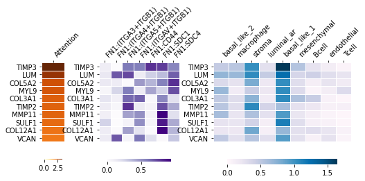
Detecting genes related specific pathways

Heatmaps for FN1 pathway related genes, and which ligand receptors affect these genes, and these FCEs come from which cell types.

_ = hn.pl.detect_pathway_related_genes(trained_MGC_model_type_GCN_list,
                                       expressed_lr_df,
                                       used_gene_list,
                                       X, adj, cell_type_names,
                                       pathway_oi='FN1',
                                       xticks_position='top')

100%|██████████| 586/586 [01:34<00:00,  6.22it/s]

Saving results for each target gene

For each target gene, saving the heatmap for LR pair attention and FCE network for LR pairs. Also saving a table including all information.

all_target_result = hn.pl.save_mgc_interpretation_for_all_target(trained_MGC_model_type_GCN_list_tmp, X, adj,
                                                                 used_genes, expressed_lr_df.reset_index(), cell_type_names,
                                                                 LR_pair_num_per_target=15,
                                                                 heatmap_plot_lr_num=15,
                                                                 edge_thres=0.2,
                                                                 save_fce_plot=True,
                                                                 palette=hn.brca_default_color_celltype,
                                                                 figures_save_folder='./_tmp_save_fig/',
                                                                 project_name='BRCA_all_target_results_tmp')

100%|██████████| 586/586 [28:26<00:00,  2.91s/it]

Model saving and loading

Trained model can be saved to avoid repetitive training. The models will be saved in ‘model_save_folder/project_name/gene_name’. The ‘gene_name’ are genes in the target_gene_name_list. For different trained model, you can set different project_name.

hn.pr.save_model_list(trained_MGC_model_type_GCN_list,
                      project_name='BRCA_10x_generating_all_target_gene_type_GCN',
                      target_gene_name_list=used_gene_list)

hn.pr.save_model_list(trained_MGC_model_only_type_list,
                      project_name='BRCA_10x_generating_all_target_gene_only_type',
                      target_gene_name_list=used_gene_list)

Setting the target_gene_name_list as one gene, the trained model for MMP11 can be saved in the same way.

Model loading. used_genes are the list of ‘gene_name’ before. Note that the order of used_genes is different from the used_gene_list before.

trained_MGC_model_only_type_list_tmp, \
used_genes = hn.pr.load_model_list(X, adj, project_name='BRCA_10x_generating_all_target_gene_only_type',
                                   only_cell_type=True)
trained_MGC_model_type_GCN_list_tmp, \
used_genes = hn.pr.load_model_list(X, adj, project_name='BRCA_10x_generating_all_target_gene_type_GCN')

Using the loaded model, you can repeat the results in the previous section.

predicted_expr_type_GCN_df_tmp = hn.pr.get_mgc_result_for_multiple_targets(trained_MGC_model_type_GCN_list_tmp,
                                                                        X, adj,
                                                                        used_genes, adata)
predicted_expr_only_type_df_tmp = hn.pr.get_mgc_result_for_multiple_targets(trained_MGC_model_only_type_list_tmp,
                                                                        X, adj,
                                                                        used_genes, adata)

100%|██████████| 586/586 [04:05<00:00,  2.38it/s]
100%|██████████| 586/586 [03:37<00:00,  2.69it/s]

only_type_vs_GCN_all2 = hn.pl.find_genes_linked_to_ce(predicted_expr_type_GCN_df_tmp.loc[:,used_gene_list],
                                                     predicted_expr_only_type_df_tmp.loc[:,used_gene_list],
                                                     used_gene_list, target_all_gene_expr,
                                                     plot_gene_list = ['MMP11'], linewidths=0.5)