Analyzing and visualizing cell-cell communication events#

In this tutorial, we demonstrate how HoloNet can be used to analyze and visualize cell-cell communication in spatial transcriptomics data.

HoloNet needs three inputs:

Spatial transcriptomic data (with gene expression matrix and spatial information).
- In this version of HoloNet, we support the spatial data based on AnnData loaded from Scanpy.
Cell-type information.
- Cell-type percentages from deconvolution methods prefer to be saved in adata.obsm['predicted_cell_type'].
- Categorical cell-type labels prefer to be saved in adata.obs['cell_type'].
Database with pairwise ligand and receptor genes.
- A pandas dataframe, must contain two columns: ‘Ligand_gene_symbol’ and ‘Receptor_gene_symbol’.

Note

The tutorial mainly follows these steps:

Load spatial transcriptomic data.
Construct multi-view communication event (CE) network among single cells (each LR pair corresponds to one view).
Visualize communication based on the multi-view network.
Other analysis methods (such as clustering LR pairs).

import HoloNet as hn

import os
import pandas as pd
import numpy as np
import scanpy as sc
import matplotlib.pyplot as plt
import torch

import warnings
warnings.filterwarnings('ignore')
hn.set_figure_params(tex_fonts=False)
sc.settings.figdir = './figures/'

Data loading#

Loading example spatial transcriptomic data#

We prepare a example breast cancer dataset for users from the 10x Genomics website. We preprocessed the dataset, including filtering, normalization and cell-type annotation. Users can load the example dataset via HoloNet.preprocessing.load_brca_visium_10x().

adata = hn.pp.load_brca_visium_10x()

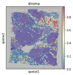
Visualize the cell-type percentages in each spot.

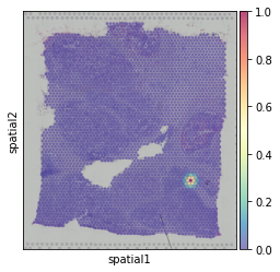
hn.pl.plot_cell_type_proportion(adata, plot_cell_type='stroma')

The figures outputed from HoloNet can be saved if adding fname parameter.

Note

The parameters of plotting functions in this tutorials are mainly inherited from two base plotting functions:

The cell-type label of each spot (the cell-type with maximum percentage in the spot)

sc.pl.spatial(adata, color=['cell_type'], size=1.4, alpha=0.7,
             palette=hn.brca_default_color_celltype)

Loading ligand-receptor database#

We provide a database with pairwise ligand and receptor genes for users. Load the database and filter the LR pairs, requiring both ligand and receptor genes to be expressed in a certain percentage of cells (or spots).

interaction_db, cofactor_db, complex_db = hn.pp.load_lr_df(human_or_mouse='human')
expressed_lr_df = hn.pp.get_expressed_lr_df(interaction_db, complex_db, adata)
expressed_lr_df.shape

(325, 12)

We also allow access to ligand-receptor pair databases based on the MITAB canonicalized nomenclature. We provide samples here so that users can import MITAB-compliant ligand-receptor databases and replace interaction_db

pd.set_option('display.max_columns', None)
interaction_db_MITAB = pd.read_csv('cellchatdb_human_interaction_example_with_MITAB.csv', index_col=0)
interaction_db_MITAB.head()

	interaction_name	pathway_name	ligand	receptor	agonist	antagonist	co_A_receptor	co_I_receptor	evidence	annotation	interaction_name_2	LR_pair	#ID Interactor A	ID Interactor B	Alt IDs Interactor A	Alt IDs Interactor B	Aliases Interactor A	Aliases Interactor B	Interaction Detection Method	Publication 1st Author	Publication Identifiers	Taxid Interactor A	Taxid Interactor B	Interaction Types	Source Database	Interaction Identifiers	Confidence Values
0	TGFA_EGFR	EGF	TGFA	EGFR	NaN	NaN	NaN	NaN	KEGG: hsa04012	Secreted Signaling	TGFA - EGFR	TGFA:EGFR	entrez gene/locuslink:1956	entrez gene/locuslink:7039	biogrid:108276\|entrez gene/locuslink:EGFR\|unip...	biogrid:112897\|entrez gene/locuslink:TGFA\|unip...	entrez gene/locuslink:ERBB(gene name synonym)\|...	entrez gene/locuslink:TFGA(gene name synonym)	psi-mi:"MI:0018"(two hybrid)	Kotlyar M (2015)	pubmed:25402006	taxid:9606	taxid:9606	psi-mi:"MI:0407"(direct interaction)	psi-mi:"MI:0463"(biogrid)	biogrid:1067440	-
1	OSM_OSMR_IL6ST	OSM	OSM	OSMR_IL6ST	NaN	NaN	NaN	NaN	KEGG: hsa04060	Secreted Signaling	OSM - (OSMR+IL6ST)	OSM:OSMR_IL6ST	entrez gene/locuslink:5008	entrez gene/locuslink:3572	biogrid:111049\|entrez gene/locuslink:OSM\|unipr...	biogrid:109786\|entrez gene/locuslink:IL6ST\|uni...	-	entrez gene/locuslink:CD130(gene name synonym)...	psi-mi:"MI:0004"(affinity chromatography techn...	Huttlin EL (2015)	pubmed:26186194	taxid:9606	taxid:9606	psi-mi:"MI:0915"(physical association)	psi-mi:"MI:0463"(biogrid)	biogrid:1176790	score:0.999999936
2	TNFSF9_TNFRSF9	CD137	TNFSF9	TNFRSF9	NaN	NaN	NaN	NaN	KEGG: hsa04060	Secreted Signaling	TNFSF9 - TNFRSF9	TNFSF9:TNFRSF9	entrez gene/locuslink:3604	entrez gene/locuslink:8744	biogrid:109817\|entrez gene/locuslink:TNFRSF9\|u...	biogrid:114281\|entrez gene/locuslink:TNFSF9\|un...	entrez gene/locuslink:4-1BB(gene name synonym)...	entrez gene/locuslink:4-1BB-L(gene name synony...	psi-mi:"MI:0004"(affinity chromatography techn...	Huttlin EL (2015)	pubmed:26186194	taxid:9606	taxid:9606	psi-mi:"MI:0915"(physical association)	psi-mi:"MI:0463"(biogrid)	biogrid:1177155	score:0.992349156
3	EFNB2_EPHB2	EPHB	EFNB2	EPHB2	NaN	NaN	NaN	NaN	PMID: 15114347	Cell-Cell Contact	EFNB2 - EPHB2	EFNB2:EPHB2	entrez gene/locuslink:1948	entrez gene/locuslink:2048	biogrid:108268\|entrez gene/locuslink:EFNB2\|ent...	biogrid:108362\|entrez gene/locuslink:EPHB2\|uni...	entrez gene/locuslink:EPLG5(gene name synonym)...	entrez gene/locuslink:CAPB(gene name synonym)\|...	psi-mi:"MI:0004"(affinity chromatography techn...	Huttlin EL (2015)	pubmed:26186194	taxid:9606	taxid:9606	psi-mi:"MI:0915"(physical association)	psi-mi:"MI:0463"(biogrid)	biogrid:1177983	score:0.999999507
4	EFNB2_EPHB3	EPHB	EFNB2	EPHB3	NaN	NaN	NaN	NaN	PMID: 15114347	Cell-Cell Contact	EFNB2 - EPHB3	EFNB2:EPHB3	entrez gene/locuslink:1948	entrez gene/locuslink:2049	biogrid:108268\|entrez gene/locuslink:EFNB2\|ent...	biogrid:108363\|entrez gene/locuslink:EPHB3\|uni...	entrez gene/locuslink:EPLG5(gene name synonym)...	entrez gene/locuslink:ETK2(gene name synonym)\|...	psi-mi:"MI:0004"(affinity chromatography techn...	Huttlin EL (2015)	pubmed:26186194	taxid:9606	taxid:9606	psi-mi:"MI:0915"(physical association)	psi-mi:"MI:0463"(biogrid)	biogrid:1177984	score:0.999990606

expressed_lr_df = hn.pp.get_expressed_lr_df(interaction_db_MITAB, complex_db, adata)

Constructing multi-view CE network#

Ligand molecules from a single source can only cover a certain region.

Before constructing multi-view communication network, we need to calculate the w_best to decide the region (‘how far is far’).

The parameters for culcalating w_best is shown in HoloNet.tools.default_w_visium().

w_best = hn.tl.default_w_visium(adata)
hn.pl.select_w(adata, w_best=w_best)

Based on w_best, we can build up the multi-view communication network.

We calculate the edge weights of the multi-view communication network. With the more attributions of ligands, HoloNet.tools.compute_ce_tensor() can set different w_best for secreted ligands and plasma-membrane-binding ligands.

Then we filter the edges with low specificities.

elements_expr_df_dict = hn.tl.elements_expr_df_calculate(expressed_lr_df, complex_db, cofactor_db, adata)
ce_tensor = hn.tl.compute_ce_tensor(expressed_lr_df, w_best, elements_expr_df_dict, adata)
filtered_ce_tensor = hn.tl.filter_ce_tensor(ce_tensor, adata, expressed_lr_df, elements_expr_df_dict, w_best)

Note

This step will consume a lot of memory. If you run out of memory, you can choose to only compute communication networks with fewer ligand-receptor pairs, and turn down the value of n_pairs parameter in HoloNet.tools.filter_ce_tensor() Also, you can set copy=False in hn.tl.filter_ce_tensor or down-sample the dataset to reduced memory consumption. When setting cut_porp as 2, we can run the whole tutorial on Macbook Pro (16G RAM, Apple M1 pro).

import random
cut_porp = 2
adata_subset = adata[random.sample(list(adata.obs_names), round(adata.shape[0] / cut_porp))]
elements_expr_df_dict = hn.tl.elements_expr_df_calculate(expressed_lr_df, complex_db, cofactor_db, adata_subset)
ce_tensor = hn.tl.compute_ce_tensor(expressed_lr_df, w_best, elements_expr_df_dict, adata_subset)
filtered_ce_tensor = hn.tl.filter_ce_tensor(ce_tensor, adata_subset, expressed_lr_df,
                                            elements_expr_df_dict, w_best, copy=False)

Visualizing CEs#

Based on the multi-view CE network, we provide two visualization methods:

CE hotspot plots for visualizing the centralities of spots. Provide two calculating methods:
- Degree centrality: out-degree + in-degree, faithfully reflects the CE strength related to each spot.
- Eigenvector centrality: reflects the core regions with active communication.
Cell-type-level CE network:
- CE strengths among cell-types

CEs hotspot plots#

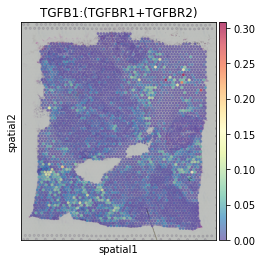
Degree centrality of each spot in the TGFB1:(TGFBR1+TGFBR2) CE network. Reflecting regions with active TGFB1:(TGFBR1+TGFBR2) communication.

hn.pl.ce_hotspot_plot(filtered_ce_tensor, adata,
                      lr_df=expressed_lr_df, plot_lr='TGFB1:(TGFBR1+TGFBR2)')

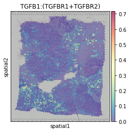
Hotspot plot based on eigenvector centrality. This plot better detects a clear center than the one based on degree centrality.

hn.pl.ce_hotspot_plot(filtered_ce_tensor, adata,
                      lr_df=expressed_lr_df, plot_lr='TGFB1:(TGFBR1+TGFBR2)',
                      centrality_measure='eigenvector')

Cell-type-level CE network#

Loading the cell-type percentage of each spot.

cell_type_mat, \
cell_type_names = hn.pr.get_continuous_cell_type_tensor(adata, continuous_cell_type_slot = 'predicted_cell_type',)

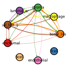
Plotting the cell-type-level CE network. The thickness of the edge represents the strength of TGFB1:(TGFBR1+TGFBR2) communication between the two cell types.

_ = hn.pl.ce_cell_type_network_plot(filtered_ce_tensor, cell_type_mat, cell_type_names,
                                    lr_df=expressed_lr_df, plot_lr='TGFB1:(TGFBR1+TGFBR2)', edge_thres=0.2,
                                    palette=hn.brca_default_color_celltype)

LR pair clustering#

Agglomerative Clustering the ligand-receptor pairs based on the centrality of each spot. The cluster label of each ligand-receptor pair saved in clustered_expressed_LR_df['cluster']. The number of clusters can be selected using n_clusters parameter in HoloNet.tools.cluster_lr_based_on_ce().

cell_cci_centrality = hn.tl.compute_ce_network_eigenvector_centrality(filtered_ce_tensor)
clustered_expressed_LR_df,_ = hn.tl.cluster_lr_based_on_ce(filtered_ce_tensor, adata, expressed_lr_df,
                                                         w_best=w_best, cell_cci_centrality=cell_cci_centrality)

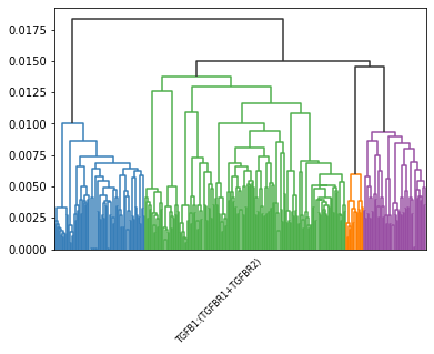
Dendrogram for hierarchically clustering all ligand–receptor pairs.

hn.pl.lr_clustering_dendrogram(_, expressed_lr_df, ['TGFB1:(TGFBR1+TGFBR2)'],
                               dflt_col = '#333333',)

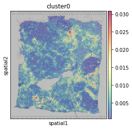
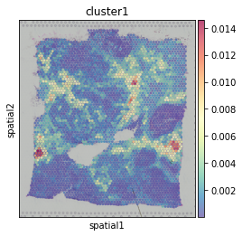
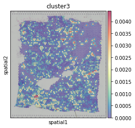
General CE hotspot of each ligand-receptor cluster (superimposing All CE hotspots of members in a cluster).

hn.pl.lr_cluster_ce_hotspot_plot(lr_df=clustered_expressed_LR_df,
                                 cell_cci_centrality=cell_cci_centrality,
                                 adata=adata)

Analyzing and visualizing cell-cell communication events

Contents

Analyzing and visualizing cell-cell communication events#

Data loading#

Loading example spatial transcriptomic data#

Loading ligand-receptor database#

Constructing multi-view CE network#

Visualizing CEs#

CEs hotspot plots#

Cell-type-level CE network#

LR pair clustering#